The all-new BeamLab 1.5 is here! This release contains some exciting new features as well as performance and stability improvements. Read on to learn what’s new or directly jump to the release notes.

Optical imaging simulations in BeamLab

Part of the BeamLab software is based on the Beam Propagation Method (BPM) which is typically used to evaluate the evolution of optical fields in free space and waveguides with rather simple input field distributions similar to those of Hermite- or Laguerre-Gaussian beams. However, in combination with complex images (e.g., the face of a wolf as shown in the example below) as input distribution, it can also be used to analyze a wide range of imaging systems incorporating lenses, apertures, optical elements that correct for aberrations or diffract the beam, and many more. BeamLab calculates the exact field distribution at any arbitrary plane between the object and image plane, and thus provides you with some unique and in-depth insights on how the imaging system works and how to optimize it.

In this respect, BeamLab 1.5 contains a couple of new features which make it very easy for you to simulate such imaging systems. For creating an input field distribution from an image file, we have added the function imageinput. It supports scaling, shifting, rotating, flipping (left-right or up-down), and inverting the image via the optional parameters Width, Shift, Rotation, FlipLeftRight, FlipUpDown, and Inverse, respectively. For example, the image wolf.png can be imported and rotated by 180° via the following simple command:

inputField = @(b) imageinput(b,'wolf.png','Rotation',180);

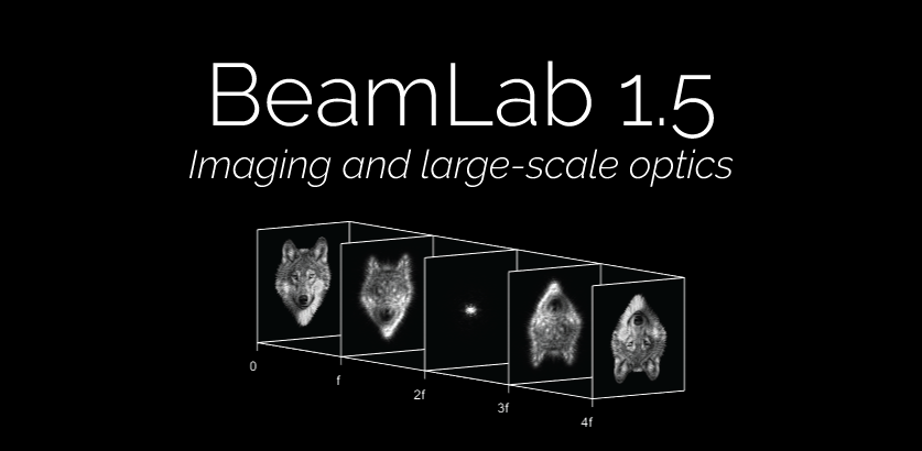
By using images as input field distributions you will be able to simulate imaging systems such as the following 4f optical system which consists of two lenses with identical focal lengths f  located at z = f and z = 3f:

Video of the light propagation in a two-lens system (4f optical system)

More slices options

Next, let’s assume you wish to add an aperture in the Fourier plane (2f-plane) of the 4f optical system to simulate an optical low-pass filter, i.e., a filter that blocks the higher spatial frequencies. In BeamLab 1.5, it is now easier than ever to display the aperture’s transmittance and the x-y intensity distribution (x-y intensity slice) directly behind the aperture by using the new optional parameters TransmittanceSlicesXY and SlicesXYSectionEnd, respectively:

apertureWidth = [50 50];
options.TransmittanceSlicesXY = true;
options.SlicesXYSectionEnd = true;

waveguide{3} = @(b) thinaperture(b,apertureWidth,options);

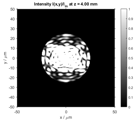
Transmittance of the thinaperture element (left) and x–y intensity slice directly behind the aperture (right)

Large-scale optics

options.OutputParameters = {'Int','Ex'};

Exciting new demos

In this release, we have also added four new imaging demos. Among those is the imaging of a pure phase object through a 4f imaging system using the principle of phase contrast microscopy. By modulating the DC (zero) spatial frequency component in the Fourier plane at z = 2f with a quarter-wave phase plate, the inherently invisible phase distribution in the object plane can be converted to a visible intensity distribution in the image plane. The following two figures show the intensity and phase distributions in the object and image planes at z = 0 mm and z = 8 mm, respectively.

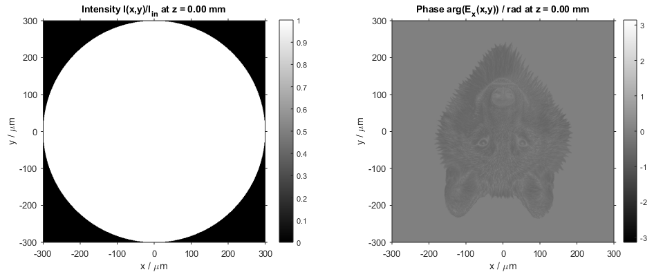
Intensity (left) and phase distribution (right) in the object plane

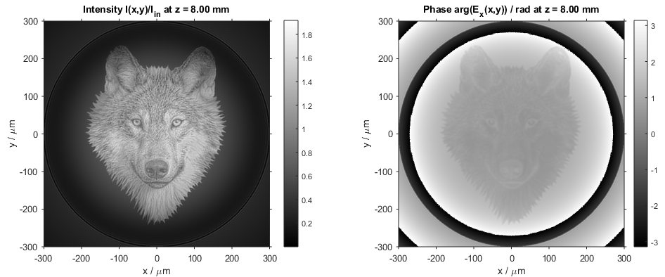
Intensity (left) and phase distribution (right) in the image plane

Interested in more examples? Please also check out our examples page.

Release notes

New features:

• Add new function imageinput, which creates an input field distribution from an image file. It supports scaling, shifting, rotating, flipping (left-right or up-down), and inverting via the optional parameters Width, Shift, Rotation, FlipLeftRight, FlipUpDown, and Inverse, respectively.
• Add new parameter OutputParameters that allows one to define which parameters are saved in the output structure at the end of the simulation.
• Add new parameter PerformanceMode that allows one to turn off refractive index scan and field monitor functions all together and thus optimize the performance of a beam propagation simulation. This new parameter has been added to all relevant demo scripts.
• Add possibility to calculate a virtual bend in multicore, plc, customwaveguide2d, and customwaveguide3d waveguides.
• Add new parameter SlicesXYSectionEnd to all waveguide functions to plot and store the field distribution appearing immediately behind a waveguide section.
• Add new parameter TransmittanceSlicesXY to thin element functions to plot and store the transmittance of a thin element.
• Add new parameter ApertureInverse to thinaperture that allows one to quickly generate and use also the inverse of the aperture function.
• Add new parameter ModeIndex that allows one to define an effective index value in whose vicinity the modes should be calculated.
• Add new parameter Polarization to modeinput to allow the usage of a Stokes (polarization) vector also in conjunction with (semi-vectorial) modes as input field.
• Add SymmetryX and SymmetryY as optional parameters to modeinput.
• Add possibility to set the optional parameters SlicesXYGraphType, SlicesXYScale, SlicesXYRange, and SlicesXYView individually for inputplot.
• Add information on the effective mode area to the output data structure of modesolver.
• Add new optional parameters MonitorScale and MonitorRange for adjusting scale and range of monitor plots independently from x-y slice plots.
• Add the possibility to use different scale and range values for each subplot in x-y, x-z, and y-z slice plots and monitor plots.
• Add function beamlabdemos, which directly opens the examples pages of the BeamLab documentation in the Help browser.

New demos:

• Add demo imaging_single_lens, which simulates the imaging of an object through a single lens with magnification M.
• Add demo imaging_single_lens_aberration, which simulates the imaging of an object through a single lens with aberrations defined via a Zernike phase screen.
• Add demo imaging_4f_system, which simulates the imaging of an object through a 4f optical system with different filter types.
• Add demo imaging_phase_contrast, which simulates the imaging of a pure phase object through a 4f optical system using the principle of phase contrast microscopy.

Enhancements:

• Improve calculation speed for fundamental modes in modesolver.
• Improve automatic assignment of ModeNumber and ModeSelect parameters.
• Improve bpmsolver, indexplot, and stacked slices plots for propagation structures containing fasthomogeneous sections.
• Improve beamoverlap to allow for input fields with different number of field components.
• Improve parsing of input parameters in beamset, inputplot, and indexplot.
• Improve 2D graphs of 2D simulations.
• Improve install function.
• Improve output structures.
• Improve titles and axis labels.
• Improve error and warning messages.
• Improve command-line output of modesolver calculations.
• Improve demo scripts.
• Improve documentation.

Parameter changes:

• Rename parameter PowerTraceType to PowerTrace.
• Rename parameter ShiftType to ShiftTransition in singlecore, multicore, plc, and rib waveguide functions.
• Rename parameter ShiftFunction to ShiftTransitionFunction in singlecore, multicore, plc, and rib waveguide functions.
• Remove parameter Monitor from thin element functions. For plotting (and storing) the transmittance of a thin element, one can now use the new parameter TransmittanceSlicesXY instead.

Bug fixes:

• Fix bug when using a function handle for indexFunction2D or indexFunction3D in customwaveguide2d or customwaveguide3d, respectively.
• Fix bug with respect to Anisotropy parameter.
• Fix bug with respect to FontSizeAxes and FontName not working correctly for 3D index contour plots.
• Various minor bug fixes.