Today, we are pleased to announce the release of our next major version BeamLab 1.3 including numerous new and (hopefully also for your application) most attractive features. Throughout the development of this release, we placed emphasis mainly on one thing: performance.
Faster than ever
BeamLab is now faster than ever since we’ve significantly improved the performance of our bpmsolver for full-vectorial calculations and for calculations using a WideAngleOrder greater than 0, a new parameter which has also been introduced in this release. The following diagram shows a comparison of the execution times of a full-vectorial BPM simulation with our demo gradedindex_waveguide for three different use cases:
- No waveguide symmetry, i.e.,
SymmetryX = falseandSymmetryY = false SymmetryX = trueSymmetryX = trueandSymmetryY = true
Thanks to the optimized algorithms, BeamLab 1.3 outperforms BeamLab 1.2 by up to a factor of 4 with respect.
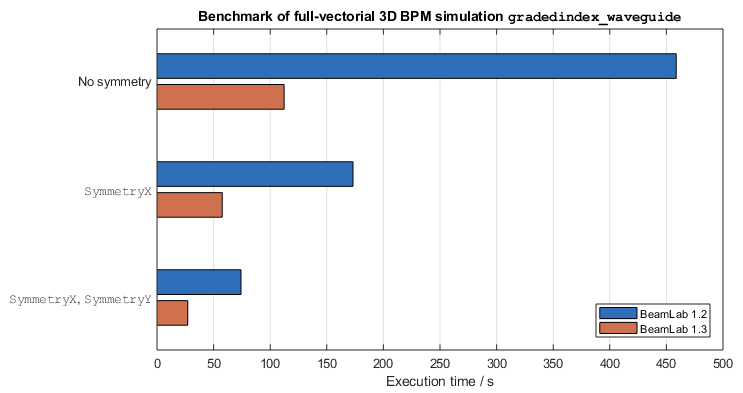
Benchmark results using an Intel® Core™ i7-7500U CPU @ 2.70GHz, 16 GB RAM, and MATLAB® version 9.3 (R2017b)
Next to these changes to bpmsolver, we’ve also significantly improved the performance of the function gaussinput and the performance of our license manager.
Not yet fast enough?
In BeamLab 1.3, we’ve also added a new waveguide function called fasthomogeneous, which opens up completely new possibilities in terms of decreasing the execution time of your simulations. Unlike the conventional function homogeneous, the new function fasthomogeneous allows you to skip entire homogeneous propagation sections by calculating in almost a twinkle of an eye the resulting field at any desired z-position thanks to an innovative combination of the beam propagation method and the angular spectrum method. For illustrative purposes, the following two figures show how fasthomogeneous can be used to replace a part of a homogeneous propagation section in order to significantly decrease the overall execution time. Since fasthomogeneous does not calculate any intermediate steps between z = 0.3 mm and 0.7 mm, this part is depicted as a white area in x–z and y–z slices.
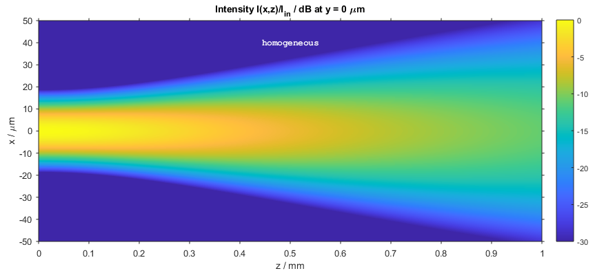
Conventional free-space beam propagation using the function homogeneous
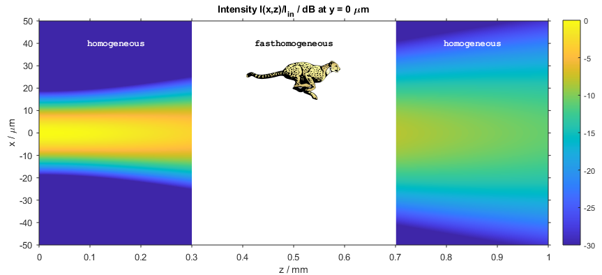
Free-space beam propagation with a fasthomogeneous section
Like any other waveguide function, fasthomogeneous can also be used together with a complex refractive index for modeling optical attenuation or gain. Furthermore, by setting the optional parameter PhaseConjugation to false or true, it is possible to quickly obtain the outcome of a forward or backward (i.e., phase-conjugate) propagation. The following figure shows the case where in the first half of the simulation a Gaussian beam is amplified while being propagated forward, whereas in the second half the amplified beam is propagated backwards to its original input state. Note that backward propagation of an amplified beam involves attenuation which is automatically taken care of.
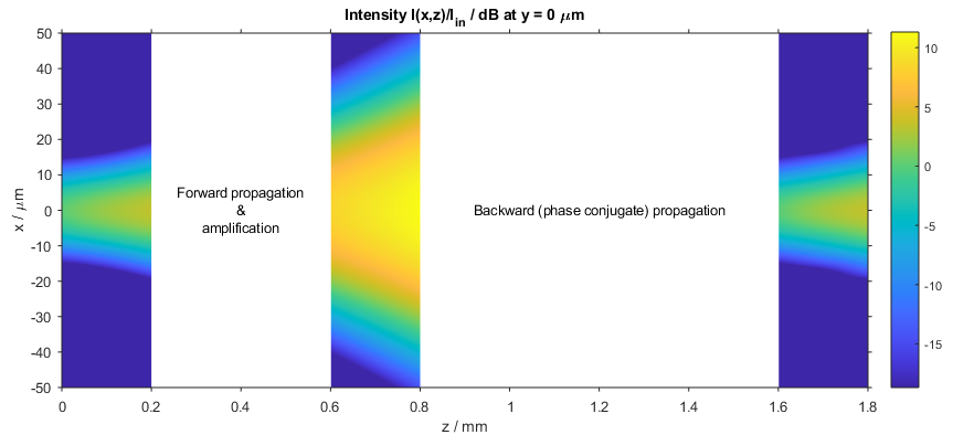
Forward and backward propagation as well as amplification and attenuation capabilities of fasthomogeneous
Exciting new demos
We’ve added two new demos, one of which shows the beam propagation in one core of a photonic lantern. The device consists of 6 cores surrounded by an inner and outer cladding tapered down to a multimode fiber where the inner and outer cladding of the photonic lantern take over the role of the core and cladding of the multimode fiber.
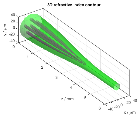
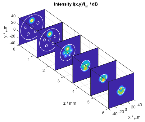
3D refractive index contour (left) and intensity profiles in the photonic lantern
Video of refractive index (left) and intensity of the beam propagating in the photonic lantern (right)
Interested in more examples? Please also check out our examples page.
Release Notes
New features:
- Add waveguide function
fasthomogeneous. This function calculates propagation through a homogeneous section in very short time. Furthermore, by using the optional parameterPhaseConjugation, one can also quickly obtain the outcome of a backward (phase-conjugate) propagation. - Add new possibilities for defining input fields. Input fields of
bpmsolverare now defined via function handles or cell arrays of function handles, which allows one to efficiently define now also multiple and superimposed input fields. For backward compatibility, it is still possible to use the old definition via field structures generated when directly calling an input field function. - Add function
inputplot, which displays the input field defined in abeamProblem. The input field to be displayed can also be specified as an input field function handle or cell array of input field function handles and passed toinputplotas second, optional parameter. Consequently, theMonitorparameters have been removed from all input field functions. - Add possibility to define complex refractive indices with negative or positive imaginary parts to all waveguide functions for modeling optical attenuation or gain. Until now, only negative imaginary parts were allowed.
- Add parameter
WideAngleOrder. This parameter allows one to specify the order of a Padé approximant up to order 3. A value of0corresponds to the Padé order (0,1) and represents paraxial approximation. Furthermore, the values1,2, and3correspond to the Padé orders (1,1), (2,2), and (3,3), respectively. The default value ofWideAngleOrderis0except forhomogeneoussections where BPM automatically adapts the algorithm for aWideAngleOrderof1. - Add parameter
ProfileExponentto the waveguide functionsplcandrib. This parameter allows one to specify the exponent of the core’s permittivity distribution to simulate various types of graded-index profiles. - Add possibility to specify
VideoResolutionin dots per inch (DPI).VideoResolutioncan now alternatively be defined as a string containing'-r'and an integer value indicating the resolution in DPI. For example,'-r300'sets the output resolution to 300 DPI. - Add demo
photonic_lantern, which simulates the beam propagation in a photonic lantern with vanishing cores. - Add demo
three_beam_interference. This demo shows how to define multiple input fields (three Gaussian beams with differentShiftandAnglevalues) that propagate simultaneously in free space.
Enhancements:
- Improve performance of
bpmsolverfor full-vectorial calculations. - Improve performance of
gaussinput. - Improve performance of license manager.
- Improve the definition of graded-index core profiles in conjunction with core shapes other than circular.
- Improve
multicorewaveguide code with respect to 2D BPM simulations. - Improve figure titles.
- Improve demo scripts.
- Improve documentation.
Bug fixes:
- Fix license manager bug when using certain MATLAB® versions.
- Fix bug when displaying the phase distribution during a BPM calculation.
- Various minor bug fixes.