Say hi to BeamLab 1.4 — another major release with some amazing new features and enhancements! This time we enhanced BeamLab to work with any input polarization state and a wide variety of anisotropic materials. Read on to learn what’s new (jump to release notes).
Arbitrary input polarizations
Beginning with this release, it is now possible to define arbitrary polarization states of input fields via a polarization vector that corresponds to the normalized Stokes vector [S1 S2 S3] with S0 = 1. When using multiple input fields, the Polarization vectors can even be defined independently from each other. For example, the following demo shows the behavior of two Gaussian beams when they cross each other in free space — in one case they have the same circular polarization defined by a Polarization vector of [0 0 1] and thus strongly interfere with each other, while in the other case they are orthogonally polarized with Polarization vectors of [0 0 1] and [0 0 -1] and do not interfere at all. With BeamLab’s simple user interface, all it takes to define these input fields is two lines of MATLAB® code:
Case 1 (same circular polarization):
inputField{1} = @(b) gaussinput(b,[30 30],'Shift',[ 30 0 0],'Angle',[-5 0],'Polarization',[0 0 1]);
inputField{2} = @(b) gaussinput(b,[30 30],'Shift',[-30 0 0],'Angle',[ 5 0],'Polarization',[0 0 1]);
Case 2 (orthogonal circular polarization):
inputField{1} = @(b) gaussinput(b,[30 30],'Shift',[ 30 0 0],'Angle',[-5 0],'Polarization',[0 0 1]);
inputField{2} = @(b) gaussinput(b,[30 30],'Shift',[-30 0 0],'Angle',[ 5 0],'Polarization',[0 0 -1]);
The following video shows the beam propagation of the two different sets of input fields:
Video of the propagation of two Gaussian beams with the same (top) and orthogonal (bottom) polarizations
Analysis of bent waveguides
We’ve also added the possibility to calculate a virtual bend in singlecore and rib waveguides. The following demo shows how the fundamental mode propagating in a silica fiber with a core index delta of 2% starts to radiate light off the core if configured as a fiber loop with a bending radius of 0.5 mm. The waveguide structure consists of 3 sections where the fiber loop (section 2) with a total length of 3.14 mm was inserted between two straight fiber sections each having a length of 1 mm.
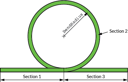
Schematic of the fiber loop
Video of the intensity profile of the beam propagating in the fiber loop
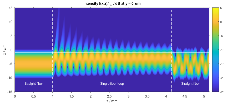
Intensity distribution in the fiber loop (x–z slice)
Propagation through anisotropic media
The possibility of defining arbitrary polarization states at the input makes it also interesting to study the change of a light wave’s polarization state when propagating through birefringent media. In the following demo, a circularly polarized Gaussian beam is first sent through a quarter-wave plate transforming the circular input polarization into a linear output polarization with the polarization plane tilted by 45°. After a short length of free-space propagation, a half-wave plate then rotates the polarization plane further from 45° to 90°, i.e., parallel to the y-axis. While the quarter-wave plate’s two principal axes are oriented in parallel to the x– and y-axis, the principle axes of the half-wave plate have been rotated by 67.5° in counter-clockwise direction to achieve the additional rotation of the polarization plane by 45°. Both wave plates have a basic refractive index of 1.5 and a thickness of 10 µm requiring a relative birefringence of 1% and 2% for the quarter-wave and half-wave plate, respectively. The wavelength used in this simulation is 0.6 µm. The whole propagation structure with five sections is defined by the following simple MATLAB® code:
indexFunction{1} = @(b) homogeneous(b,2,1);
indexFunction{2} = @(b) homogeneous(b,10,1.5,'Anisotropy',[1 1.01 1]);
indexFunction{3} = @(b) homogeneous(b,2,1);
indexFunction{4} = @(b) homogeneous(b,10,1.5,'Anisotropy',[1 1.02 1],'Rotation',67.5);
indexFunction{5} = @(b) homogeneous(b,2,1);
Video of the beam propagating through a quarter-wave and a half-wave plate
Interested in more examples? Please also check out our examples page.
Release notes
New features:
- Add the possibility to define the input polarization via a polarization vector (i.e., normalized Stokes vector) that allows one to work with arbitrary input polarizations. In this respect, the
Polarizationparameter has been moved frombeamsetto the input field functions. Both semi-vectorial and full-vectorial BPM calculations can be performed with arbitrary input polarizations. For semi-vectorial mode calculations the desired polarization can be set via the new parameterModePolarization. - Add information on the E-field’s polarization state at the x-y slices and output plane to the output data structure of a BPM calculation.
- Add the possibility to calculate a virtual bend in
singlecoreandribwaveguides. - Add possibility to define the anisotropy of waveguides by means of a 3- or 5-element vector representing the relative components
[xx,yy,zz]or[xx,yy,zz,xy,yx]of the index tensor. - Add new optional parameters
AnisotropyCore,AnisotropySubstrate, andAnisotropyCladdingtorib, replacing the single parameterAnisotropy. This allows one to define the refractive index anisotropy for core, substrate, and cladding individually. - Add two new options
'DvsLambda'and'DvsV'to the parameterDispersionGraphTypefor plotting the dispersion parameter D as a function of wavelength and normalized frequency, respectively. - Add scale options
'lincustom'and'logcustom'to parametersSlicesXYScale,SlicesXZScale,SlicesYZScale, andPowerTraceScale. The new scale options allow one to define a linear or logarithmic scale, respectively, normalized to a custom value. In case ofSlicesXYScale,SlicesXZScale, andSlicesYZScale, this custom value is defined by the new optional parameterSlicesCustomNormand in case ofPowerTraceScale, the custom value is defined by the newly added parameterPowerCustomNorm. - Add possibility to address simultaneously an arbitrary ensemble of cores with
ModeCoreand thus calculate the (super)modes defined by these cores. - Add new optional parameter
ModeSelectthat allows one to select specific modes (either in form of a scalar or a vector) out of a larger mode ensemble. - Add the possibility to define
modesolverrelevant parameters such asModeCore,ModeNumber,ModePolarization,ModeSections,ModeSelect, andModeSortingOrderdirectly as input parameters ofmodeinput. In addition,modeinputnow also allows one to define an input distribution that consists of a linear combination of modes with different mode amplitudes by assigning a vector containing the relevant mode numbers toModeSelectand a vector containing the appropriate mode amplitudes toModeAmplitude. - Add new optional parameter
Phaseto all input field functions for specifying the input field’s phase in degrees. - Add possibility to display phase and index distributions in x-z and y-z slices.
- Add possibility to display multiple x-z and y-z slice plots of different types.
- Add new optional parameter
QuiverLengththat allows one to adjust the length of the quiver arrows. - Add new optional parameter
ShowSectionTitlesfor displaying section titles inside the figure during monitor. The position inside the figure can be specified by the new parameterSectionTitlePosition. - Add option to
beamlabdocfor searching the documentation for pages with words matching a specified expression. - Add demo
fiber_loop, which simulates the propagation of the fundamental mode of a fiber through a fiber loop. - Add demo
fiber_bend_modes, which calculates the first three eigenmodes of a fiber with a bending radius of 10 cm. - Add demo
fiber_bend_loss, which calculates the bending loss of the first three eigenmodes of a fiber with a bending radius of 10 cm as a function of the wavelength. - Add demo
quarterwave_plate, which simulates the propagation of a Gaussian beam with circular polarization through a quarter-wave plate. - Add demo
noninterfering_beams, which simulates the propagation of two orthogonally polarized Gaussian beams that cross each other in free space. - Add demo
fiber_taper, which simulates the propagation of the fundamental mode of a fiber whose size is changed by means of a fiber taper.
Enhancements:
- Eliminate the need for the user-defined parameters
FieldSymmetryXandFieldSymmetryY. Field symmetries are now set automatically according to the input field and index symmetriesSymmetryXandSymmetryY. - Extend full-vectorial
bpmsolverto work also with anisotropichomogeneousandsinglecorewaveguides that are rotated by some arbitrary angle. - Improve power area definition. The
SmoothingLevelparameter is now also used for smoothing the rim of the power area. - Improve display of quiver arrows in x-y slice plots.
- Improve performance of license manager.
- Improve demo scripts.
- Improve documentation.
Bug fixes:
- Fix bug in
dispersionsolverwhen using cores with index trenches. - Fix bug in
indexplotwhen usingfasthomogeneoussections. - Fix bug when modeling a tapered
ribwaveguide. - Fix license manager bug when using macOS or Linux.
- Various minor bug fixes.