Welcome to BeamLab 2.4! We are pleased to announce our latest release where we focused mainly on performance and stability improvements. Read on to learn about how to evaluate the dispersion properties of optical fibers with BeamLab (or directly jump to the release notes).

Evaluating the dispersion properties of optical fibers with BeamLab

Nearly every bit of digital data that we consume nowadays when accessing information via the Internet passes through an optical fiber in form of optical pulses somewhere on its way from its source to its destination. An optical fiber is made from either silica glass or plastic. A core, with a typically slightly higher refractive index than the surrounding cladding, guides the information-carrying light pulses over many kilometers without significant attenuation. The light guiding and dispersion properties of an optical fiber are mainly determined by the core’s refractive index profile. The types of fibers used in optical fiber communications can be broadly classified into step-index fibers and graded-index fibers. The former has a core with a constant refractive index across a width of less than 10 μm and typically guides only a single spatial mode to enable long-haul communications at very high data rates. The latter has a core with a (nearly) parabolic refractive index profile across a width of a few 10 to about 100 μm which lets the input light pulse spread across multiple spatial modes. Coupling light into a multimode fiber with a larger core is easier and hence multimode fiber systems are less expensive to build and operate. On the other hand, exciting multiple modes with different propagation properties causes modal dispersion and makes the transmission of high data rates over long distances difficult unless special receiver techniques are used to untangle the mode mixing and compensate for the different delays that modes undergo while propagating in the fiber. This typically makes the multimode fiber more suitable for short-range communications, e.g., inside buildings or vehicles.

With optical fibers being ubiquitous in today’s telecommunications infrastructure, it is essential to have a simulation tool at hand that allows one to characterize their properties easily and quickly. BeamLab is equipped with a solver, dubbed dispersionsolver, that exactly fulfills this task. This blog presents a quick guide to the main features of dispersionsolver. Based on the two-dimensional refractive index distribution defining the cross-section of an optical fiber, dispersionsolvernot only calculates the propagation constants of all propagating modes within a user-defined range of wavelengths, but also derives thereof various dispersion properties such as the modes’ group delays, chromatic dispersion, effective areas etc.

Figure 1 depicts a graph that is often found in textbooks on optical fibers and probably familiar to many readers of this blog as well. It shows the dependence of the fiber modes’ normalized propagation constants B on the normalized frequency V. Such a graph can be easily generated with dispersionsolver. In this example we used a step-index core with a core diameter of 8 μm and a relative core-cladding index difference of 0.4% representing a standard single mode fiber at the wavelength of 1.55 µm. V is plotted from 2 to 6, corresponding to a wavelength range from about 1.63 μm down to 0.55 μm. The figure on the left shows the propagation constants of the fiber’s true modes (also known as the HE and EH modes), while the figure on the right shows the fiber’s LP modes. The LP modes are linear polarized modes formed by grouping together true modes with similar propagation characteristics. LP modes are often used as a simplified representation of the true modes under the assumption of a sufficiently small index difference between core and cladding. In BeamLab, the LP modes are calculated by setting the beamset parameter VectorTypeto 'semivectorial'. For a relative core-cladding index differences of less than a few percent, as being used for most practical optical fibers, the differences in propagation constants between the two plots are hardly recognizable unless one zooms in on a small section of the curve pertinent to, e.g., the first higher-order mode group, which consists of the TE₀₁, TM₀₁, HE_21x and HE_21y modes in case of the (full-vectorial) true mode plot on the left, and the LP_11a und LP_11b modes in case of the (semi-vectorial) LP modes on the right, as shown by the insets. For reference purposes, the intensity distributions of the individual modes were separately calculated with BeamLab’s modesolver at V = 6 (λ ≈ 0.55 μm) and are displayed next to the right vertical axis of each figure.

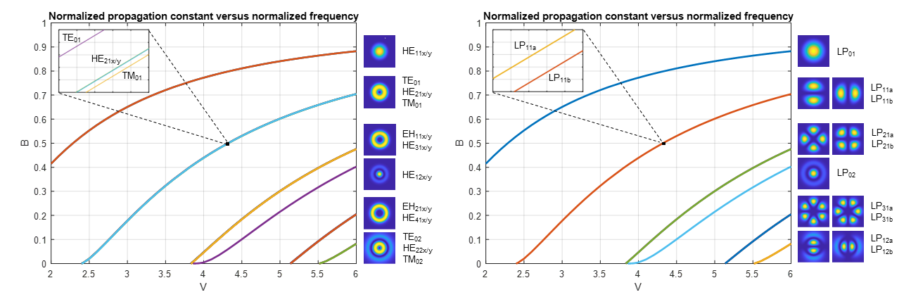
Fig. 1: Normalized propagation constant B versus normalized frequency V for true modes (left) and LP modes (right) of a step-index fiber

For the sake of simplicity, in the remainder of the blog we use only the LP modes. The type of dispersion characteristics to be plotted by dispersionsolver is defined in the beamset parameter DispersionEvaluationType. Independent of its contents, however, once a dispersion calculation has completed over the user-defined range of wavelengths or normalized frequencies, any dispersion characteristic that is available through DispersionEvaluationType can be immediately generated by using the function dispersionplot and the output data of a previous dispersionsolver calculation as well. For example, the plots shown in Fig. 2 could be generated with dispersionplot by using the output data of the above-mentioned calculation as its input parameter and additionally setting the optional parameter DispersionEvaluationType to the desired type of dispersion characteristics. For the following figure we chose the dispersion parameter D (chromatic dispersion) and effective area A_eff. Furthermore, we selected only the lowest-order three modes (LP₀₁ and LP_11a/b) to be displayed by setting the dispersionplot parameter ModeSelect to [1 2 3]. The left plot shows the chromatic dispersion, and the right plots shows the effective area as a function of wavelength of all three modes within the wavelength range from 1 to 1.6 μm. The effective area is a field distribution dependent weighted average of the area that is occupied by each mode and is often used as a measure of the mode’s response to nonlinear effects. Higher-order modes typically have larger effective areas and are thus also less prone to nonlinear effects.

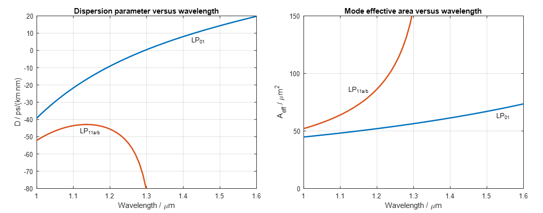
Fig. 2: Dispersion parameter D (left) and effective area A_eff (right) versus wavevlength of a step-index fiber

For our second example, we chose a graded-index fiber with a core diameter of 30 μm and a perfect parabolic refractive index profile in the core with a core-cladding index difference of 1%. Figure 3 shows the normalized propagation constant on the left, but this time as a function of wavelength for the wavelength range from 1 to 1.6 μm, and the modes’ differential group delays (or modal delays) on the right.

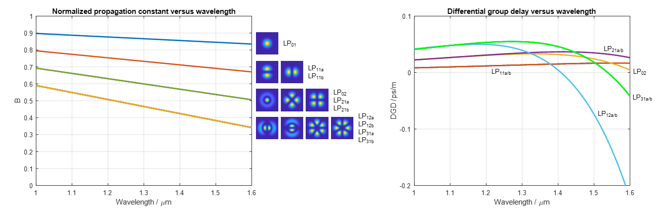
Fig. 3: Normalized propagation constant B (left) and differential group delay DGD (right) versus wavelength of a graded-index fiber

Finally, we note that dispersionsolver not necessarily requires a range of wavelengths or normalized frequencies to be defined to calculate certain dispersion properties. A range is only required if an output in form of a dispersion plot is desired as shown in the above figures. For example, if only the mode field diameter of the fundamental mode at a single wavelength, e.g., 1.3 μm, is of interest, simply insert the single wavelength value into the DispersionScanVector parameter, or leave the parameter empty and instead set the beamset parameter lambda to the wavelength of your choice.

Below is a list of parameters that can be evaluated with dispersionsolver :

• 'Aeff'  Effective area
• 'B'  Normalized propagation constant
• 'D'  Dispersion parameter (chromatic dispersion)
• 'Deff'  Effective diameter (derived from 'Aeff')
• 'DGD'  Differential group delay
• 'DS'  Dispersion slope
• 'GD'  Group delay
• 'GVD'  Group velocity dispersion
• 'MFD1'  Mode field diameter defined by Petermann I equation
• 'MFD2'  Mode field diameter defined by Petermann II equation
• 'Neff'  Effective refractive index
• 'Ngroup'  Group index

Release notes

New features:

• Add new parameter PowerCore to waveguide functions multicore, plc and rib to allow one to select individual cores for a power trace.
• Add new parameter DzData to waveguide function importedwaveguide3d to allow one to define the distance between individual refractive index slices also if the waveguide data is defined as a 3D array.
• Add possibility to evaluate the dispersion slope DS and group velocity dispersion GVD with dispersionsolver.

Modified functions:

• The variable used to describe the distance between individual refractive index slices in importedwaveguide3d, when the waveguide data is given by a MAT-file, has been renamed to dzData.

Modified demos:

• Add an example on the use of the new parameter PowerCore to the demo multicore_index_trench.

Enhancements:

• Improve beamoverlap to enable the calculation of the overlap integral between an E- and H-field.
• Improve the accuracy in emulating bent waveguides by means of the waveguide functions singlecore, multicore, plc and rib.
• Improve warning and error messages.
• Improve documentation.

Bug fixes:

• Fix bug in modesolver.
• Fix bug in indexplot.
• Fix bug in importedwaveguide3d.
• Various minor bug fixes.