Welcome to BeamLab 2.2! We are pleased to announce our latest release which is packed with exciting new features as well as performance and stability improvements. Read on to learn more about some of the highlights or directly jump to the release notes.
Creating a waveguide’s refractive index distribution via an image file
One of BeamLab’s strengths is a simple user-interface that does not require the user to learn how to use a proprietary CAD tool to set up the simulation model. As such, BeamLab comes with a large number of pre-defined waveguide functions to enable a quick and easy setup of basic waveguide structures such as tapers, splitters, couplers, etc. Although these functions and their combinations cover a wide range of applications, it is also clear that they could never fulfill the design needs with respect to all thinkable waveguide structures. To break through a potential design limitation based on pre-defined functions and thus provide our users with greater flexibility in designing and simulating the waveguides of their choice, we added this time a new waveguide function dubbed importedwaveguide that allows one to import and create waveguides based on a two-dimensional image representing the refractive index distribution of the waveguide’s cross-section in either the x-y, x-z, or y-z plane. In the following example, we show the refractive index contour and respective field propagation through a planar waveguide representing the input star coupler of an arrayed waveguide grating that was created by means of a black & white PNG image drawn with a third-party CAD software and imported into BeamLab. In this specific example the image represents the waveguide’s cross-section in the x-z plane. The waveguide’s thickness was separately defined by the optional parameter Width of the function importedwaveguide to be 2 µm.
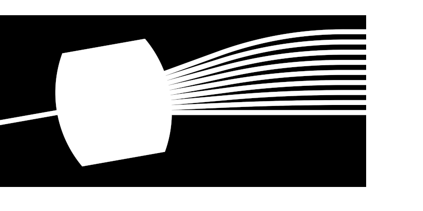
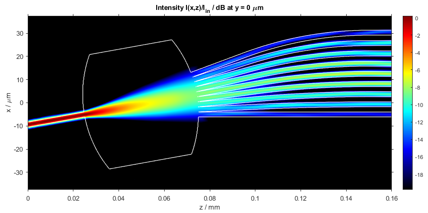
PNG image (left) and two-dimensional intensity distribution (right)
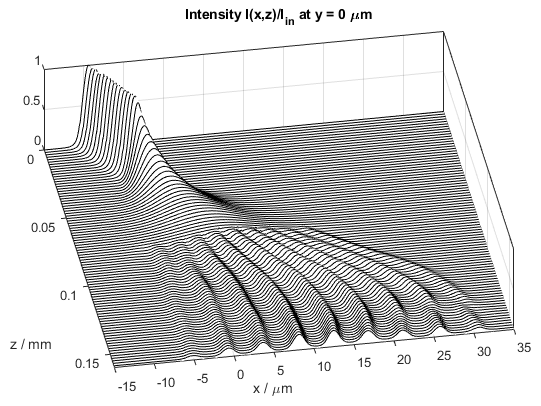
Three-dimensional intensity distribution displayed with black mesh lines (illustrating BeamLab’s extensive plot capabilities)
Cascading simulations with different grid sizes and resolutions
A simulation model in which the lateral extension of the propagation beam varies by a large factor, e.g., hundred or more, can be computationally very expensive as the resolution for the whole model needs to be set according to the smallest extension or feature. In this release we added a function dubbed resizefield that allows one to easily adjust the size and resolution of the output field of the previous calculation to the size and resolution of the next one and thus optimize calculation speed without sacrificing accuracy. In the following example, we illustrate this by focussing a collimated Gaussian input beam with a beam width of 1 mm into a waveguide core with a width of 5 µm by using a thin lens with a focal length of 2.5 mm. By splitting the simulation model into multiple sections, the grid size is gradually reduced from 2 mm to 60 µm and thus optimized to cover just the area where the beam’s field strength is mostly concentrated and significant enough to affect the propagation characteristics.
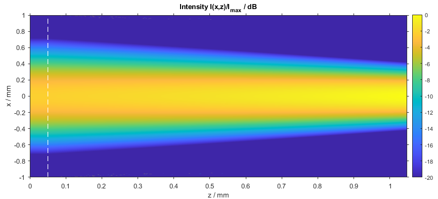
Intensity distribution of 1st section (lateral size: 2 mm, length: 1.05 mm) including a thin lens at z = 0.05 mm
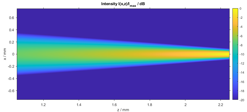
Intensity distribution of 2nd section (lateral size: 1.5 mm, length: 1.2 mm)
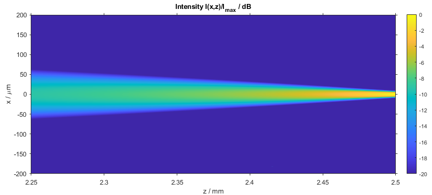
Intensity distribution of 3rd section (lateral size: 0.4 mm, length: 0.25 mm)
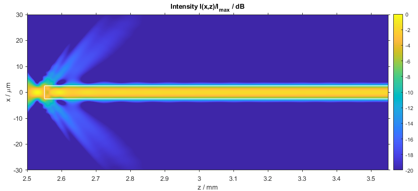
Intensity distribution of 4th section (lateral size: 0.06 mm, length: 1.05 mm) including the waveguide
Calculating the electric and magnetic field simultaneously
Algorithms based on the beam propagation method mostly focus on the calculation of the electric field. However, for an accurate evaluation of the power flow throughout the simulation model it is essential to have also knowledge on the real part of the Poynting vector which in turn requires also knowledge of the magnetic field. Starting with this release, BeamLab offers the possibility to calculate the electric and magnetic field simultaneously and thus provides a means for the accurate evaluation of the Poynting vector. If the parameter FieldType is set to 'EH', any intensity related calculation will be automatically based by default on the real part of the Poynting vector.
Exciting new demos
In this release we also expanded significantly our demo library. One of the new demos is dubbed nanf and gives an example on how to calculate the eigenmodes of a nested antiresonant nodeless hollow core fiber (NANF). Among the various types of photonic crystal fibers developed so far, NANFs have attracted considerable attention in recent years for their potential to achieve for the first time a lower propagation loss over a broader wavelength range than conventional solid core fibers. The following figures depict the NANF’s cross-sectional refractive index and fundamental mode’s intensity distribution, respectively.
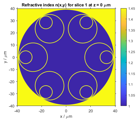
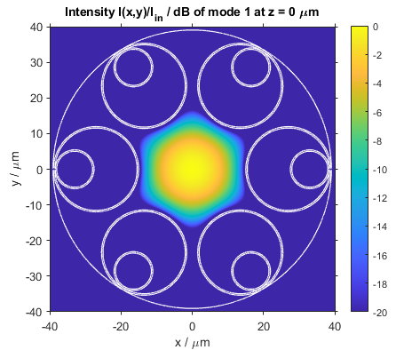
Refractive index distribution (left) and intensity distribution of the fundamental mode (right)
Another demo dubbed metal_slit illustrates how BeamLab works with media that exhibit a complex refractive index such as metals. In this demo a metal slit made from Aluminium is illuminated with a Gaussian beam in width twice that of the slit. The following figures show the intensity distribution in the x-z plane for the cases where the input beam exhibits y (or TE) polarization and x (or TM) polarization, respectively.
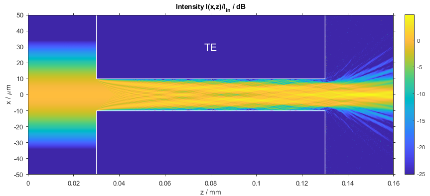
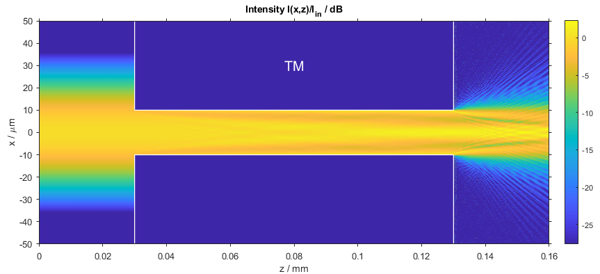
Intensity distribution of TE-polarized (left) and TM-polarized (right) light propagating through a metal slit
Finally, a third demo that we would like to introduce here is the demo dubbed ronchi_grating_thick which depicts the field changes in close vicinity of a “thick” (in contrast to thin elements of zero thickness) Ronchi grating. The refractive index of the substrate is 1.5 and the grating’s groove depth is chosen to generate a phase delay of π . The following figure shows the field distribution of the electric field’s real part in the x-z plane. At the grating’s output plane the beam’s phase alternates between 0 and π . The generation of such thick gratings whose thickness, surface profile and refractive index of the unit cell can be freely defined by the user is now enabled by the new function grating.
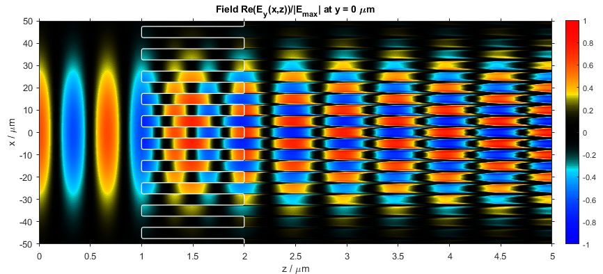
Field distribution in close vicinity of a Ronchi grating illuminated by a Gaussian beam from the substrate side
Release notes
New features:
- Add new function
importedwaveguide. This function allows one to create a waveguide whose x-y, x-z, or y-z refractive index distribution is externally generated and imported by means of a matrix or an image file. - Add new function
gratingwhich emulates a grating whose thickness, surface profile and unit cell refractive index distribution is defined by the user. - Add possibility to calculate simultaneously the electric and magnetic field by specifying the new value
'EH'inFieldType. - Add possibility to use the parameter
UseParallelin conjunction withmodesolverto speed up mode calculations when the refractive index distribution is symmetric with respect to the x- and/or y-axis. - Add possibility to set
QuiverPeriodin x- and y-direction independently. - Add possibility to define the parameter
WideAngleOrderindividually in each section. - Add new function
resizefield. This function adapts the resolution of a field distribution from one bpmsolver calculation to the next. - Add new parameter
SlicesXYPlotXYStepthat allows one to adjust the plot resolution in the x-y plane of all field and monitor x-y plots. - Add new parameters
IndexSlicesXZ,IndexSlicesXZGraphType,IndexSlicesYZandIndexSlicesYZGraphTypetoindexplotthat allow one to generate x-z and y-z plots of the refractive index distribution. - Add new parameters
CoreRotationandCoreRotationEndto waveguide functionmulticoreto allow one to rotate the cores of each core ring independently of the total waveguide rotation. - Add new parameter
AnisotropyRotationTransitionto waveguide functionssinglecoreandmulticoreto define the way the orientation of the anisotropy changes fromAnisotropyRotationtoAnisotropyRotationEnd. - Add new parameter
RotationTransitionto waveguide functionsinglecoreto define the way the core rotation angle changes fromRotationtoRotationEnd. - Add new parameters
Angle,Polarization, andPowertoimageinputin accordance with the other input field functions.
New or modified demos:
- Add demo
awgwhich shows the beam propagation through the input star coupler of a simplified arrayed waveguide grating. - Add demo
waveguide_couplerwhich shows an example on how to use the new functionresizefieldto simulate the coupling of a Gaussian beam with a beam width of 1 mm to a waveguide with a core width of 5 um. - Add demo
nanfwhich calculates the field distributions and effective refractive indices of the eigenmodes of a nested antiresonant nodeless fiber. - Add demo
metal_slitwhich shows the beam propagation through a metal slit for both TE and TM polarization. - Add demo
photonic_lantern_modeselectivewhich shows the beam propagation through two mode-selective photonic lanterns in a back-to-back configuration. - Add demo
fiber_anglepolishedwhich shows the beam propagation through a single-mode fiber that is terminated with an 8 degree angle-polished (slanted) end face. - Add demo
fiber_loop_adiabaticwhich shows the beam propagation through a fiber loop with an adiabatic bend radius transition. - Add demo
ronchi_grating_thickwhich shows the beam propagation through a thick Ronchi phase grating. - Add demo
blazed_gratingwhich shows deflection of a Gaussian beam when propagating through a blazed phase grating. - Rename demo
ronchi_gratingtoronchi_grating_thin. - Rename demo
fiber_looptofiber_loop_abrupt.
Enhancements:
- Improve the performance of
modesolvercalculations. - Improve warning and error messages.
- Improve documentation.
Parameter changes:
- Rename parameter
CalculationCentertoOrigin. In addition to defining the calculation origin in the x-y plane, this parameter now allows one to define also the z-coordinate of the calculation origin. In other words, the calculation origin does not necessarily need to be[0,0,0]but can be set to any location in the three-dimensional space. - Rename parameter
RingAngleOffsettoRingAngleinmulticore. - Rename parameter
RingAngleTransitiontoRotationTransitioninmulticore.RotationTransitiondefines the transition of the rotation angle fromRotationtoRotationEnd,RingAngletoRingAngleEndandCoreRotationtoCoreRotationEnd.
Bug fixes:
- Fix bug in input functions
uniforminput,imageinput, andgaussinput. - Fix bug in
thinapertureandthinlens. - Fix bug when displaying quiver arrows in field plots using the parameter
Quiver. - Fix bug with respect to parameter
SlicesXZYZPlotXYStep. - Various minor bug fixes.